

Scalar: the heart of computational graphs#
In mlfz, computational graphs are implemented by the Scalar class. (And also the Tensor class, but to flatten the learning curve, we’ll stick to vanilla
computational graphs without vectorization.)
You can think about Scalar as a number that keeps track the computations that yielded it. We instantiate a one by either setting its value or using operations and functions on other Scalar’s.
from mlfz.nn.scalar import Scalar

a = Scalar(3)
b = Scalar(-2)

a + b
Scalar(1)
You can even randomly initialize a Scalar via the Scalar.from_random method.
Scalar.from_random()
Scalar(0.5149408215492743)
As Scalar represents a node in a computational graph, each one holds
a numeric value,
the backwards gradient (whatever that might be),
and the list of incoming edges.
Let’s see these on the simple example of a * b.
a = Scalar(3)
b = Scalar(-2)

c = a * b
c.value
-6
We’ll talk about the backwards gradient in detail when we discuss backpropagation and the backward pass. For now, its value is 0, but it’ll contain the derivative of the loss function with respect to the node.
c.backwards_grad
0
The Scalar.prevs attribute contains a list of Edge objects, each representing an incoming edge.
c.prevs
[Edge(prev=Scalar(3), local_grad=-2), Edge(prev=Scalar(-2), local_grad=3)]
In turn, each edge contains
a
Scalar,and the derivative of the children node, given the parent node.
edge_a_c = c.prevs[0]
edge_a_c.prev
Scalar(3)
In our case, the local gradient equals to \( \frac{\partial c}{\partial a} = b \), which is \( -2 \) in this example.
edge_a_c.local_grad
-2
Essentially, Scalar is a wrapper over a number. That’s why functions like Python’s built-in sum work on them:
sum([Scalar(1), Scalar(2)])
Scalar(3)
Let’s see how to build computational graphs!
Defining computational graphs#
As you can see, the Scalar class is overloaded with features: it dynamically builds the underlying computational graph without you having to worry about it. Let’s see an example.
a = Scalar(3)
b = Scalar(-2)
x = Scalar(0.5)

y = a * x + b
The expression a * x + b describes a directed graph with nodes a, b, a * x, x, and a * x + b. It’s easier to draw a picture.
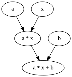
In mlfz, the computational graph is fully represented by Scalars and Edges. All you need to do is to define functions using operations and functions as building blocks. Scalar objects are compatible with addition, subtraction, multiplication, division, and exponentiation; that is, the operators +, -, *, /, and **.
Besides those, the mlfz.nn.scalar.functional module contains functions like sin, cos, exp, and log.
from mlfz.nn.scalar.functional import sin, cos


x = Scalar(-4.6)
y = Scalar(1.3)

sin(x) + cos(y)
Scalar(1.2611898322580517)
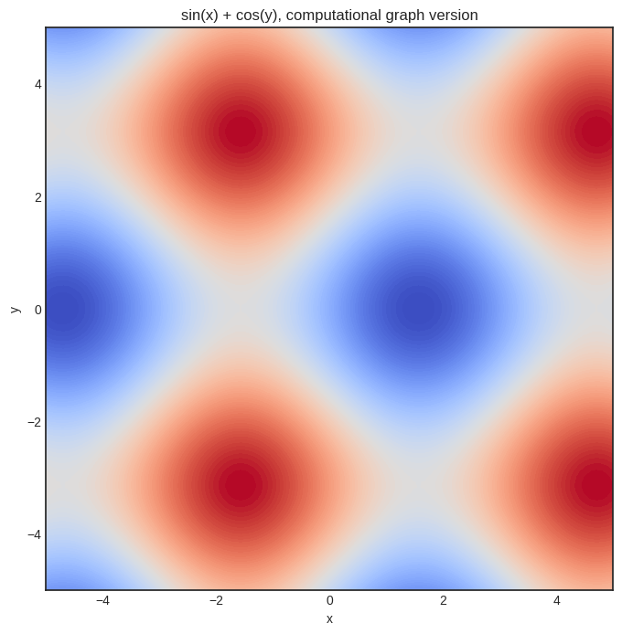
Just to convince you that it works, here’s the plot of our sin(x) + sin(y) function.
Show code cell source
import matplotlib.pyplot as plt
import numpy as np


with plt.style.context("seaborn-v0_8-white"):
    plt.figure(figsize=(8, 8))

    res = 100
    x = np.linspace(-5, 5, res)
    y = np.linspace(-5, 5, res)
    xx, yy = np.meshgrid(x, y)

    zz = np.vectorize(lambda x, y: (sin(Scalar(x)) + cos(Scalar(y))).value)(xx, yy)

    plt.contourf(xx, yy, zz, levels=100, cmap='coolwarm_r')
    plt.xlabel('x')
    plt.ylabel('y')
    plt.title('sin(x) + cos(y), computational graph version')
    plt.show()
The backward pass#
To get a node’s derivative with respect to all preceding nodes, we use the famous backpropagation algorithm, implemented via the Scalar.backward method.
Let’s see it in action!
x, y = Scalar(1.2), Scalar(-6.9)
z = (sin(x) + cos(y))**2

z.backward()
Recall the mysterious Scalar.backwards_grad attribute? This is where z’s derivatives are stored! Upon calling z.backward(), the derivatives are calculated with respect to all preceding nodes, and then stored in the backwards_grad attribute.
Let’s see \( \frac{\partial z}{\partial x} \)!
x.backwards_grad
1.2666318116545192
What about \( \frac{\partial z}{\partial y} \)?
y.backwards_grad
2.021952608019056
As
we can check the correctness via Python’s built-in trigonometric functions from the math module.
from math import sin as sin_vanilla, cos as cos_vanilla

def z_grad(x, y):
    return (2 * cos_vanilla(x) * (sin_vanilla(x) + cos_vanilla(y)),
            -2 * sin_vanilla(y) * (sin_vanilla(x) + cos_vanilla(y)))

z_grad(x.value, y.value) == (x.backwards_grad, y.backwards_grad)
True
Yay!
Scalar is pretty simple to use; that was more or less all about it. In the next part, we’ll use computational graphs to train our first machine learning model: a linear regression. Let’s get to it!