Building a vectorized neural network with tensors#
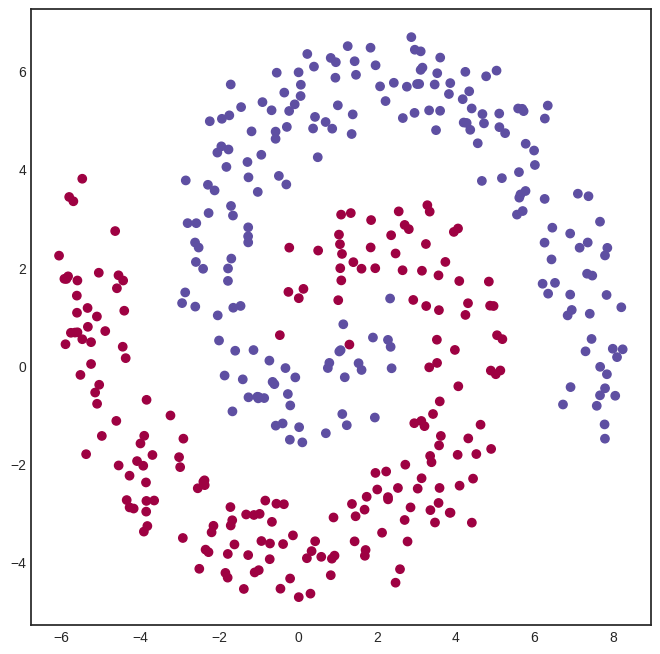
To demonstrate the power of Tensor, we’ll need a dataset to test out our neural network. We’ll use our good old friend, the spiral dataset.
Show code cell source
import numpy as np
from mlfz.nn import Tensor


def generate_spiral_dataset(n_points, noise=0.5, twist=380):
    random_points = np.sqrt(np.random.rand(n_points)) * twist * 2 * np.pi / 360

    class_1 = np.column_stack((-np.cos(random_points) * random_points + np.random.rand(n_points) * noise,
                               np.sin(random_points) * random_points + np.random.rand(n_points) * noise))
    class_2 = np.column_stack((np.cos(random_points) * random_points + np.random.rand(n_points) * noise,
                               -np.sin(random_points) * random_points + np.random.rand(n_points) * noise))

    xs = np.vstack((class_1, class_2))
    ys = np.hstack((np.zeros(n_points), np.ones(n_points))).reshape(-1, 1)

    return Tensor(xs), Tensor(ys)
xs, ys = generate_spiral_dataset(200, noise=2)
Show code cell source
import matplotlib.pyplot as plt


with plt.style.context("seaborn-v0_8-white"):
    plt.figure(figsize=(8, 8))
    plt.scatter([x[0] for x in xs], [x[1] for x in xs], c=ys, cmap=plt.cm.Spectral)
    plt.show()
To define a network, we’ll once again use the Model class from mlfz.nn.
from mlfz.nn import Model
from mlfz.nn.tensor.functional import tanh, sigmoid


class TwoLayerNetwork(Model):
    def __init__(self):
        self.A = Tensor.from_random(2, 8)
        self.B = Tensor.from_random(8, 8)
        self.C = Tensor.from_random(8, 1)

    def forward(self, x):
        return sigmoid(tanh(tanh(x @ self.A) @ self.B) @ self.C)

    def parameters(self):
        return {"A": self.A, "B": self.B, "C": self.C}
Look at how simple this implementation is, compared to the scalar version. Writing expressions like tanh(x @ A) makes all the difference.
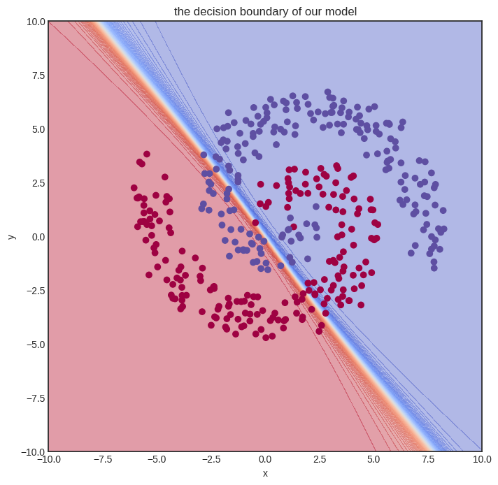
Training tensor networks is also much faster, as we shall see soon. Let’s initialize one and see how it looks.
model = TwoLayerNetwork()
Show code cell source
from itertools import product


def visualize_model(model, xs, ys, res=100, xrange=(-10, 10), yrange=(-10, 10)):
    with plt.style.context("seaborn-v0_8-white"):
        plt.figure(figsize=(8, 8))

        res = 100
        x = np.linspace(xrange[0], xrange[1], res)
        y = np.linspace(yrange[0], yrange[1], res)
        xx, yy = np.meshgrid(x, y)
        zz = np.zeros_like(xx)

        for i, j in product(range(res), range(res)):
            zz[i, j] = model.forward(Tensor([xx[i, j], yy[i, j]])).value


        # plot the decision boundary
        plt.contourf(xx, yy, zz, levels=100, cmap='coolwarm_r', alpha=0.4)
        plt.xlabel('x')
        plt.ylabel('y')
        plt.title('the decision boundary of our model')

        # plot the data
        plt.scatter([x[0] for x in xs], [x[1] for x in xs], c=ys, cmap=plt.cm.Spectral, zorder=10)
        plt.show()

visualize_model(model, xs, ys)
/tmp/ipykernel_1198/4170422174.py:15: DeprecationWarning: Conversion of an array with ndim > 0 to a scalar is deprecated, and will error in future. Ensure you extract a single element from your array before performing this operation. (Deprecated NumPy 1.25.)
  zz[i, j] = model.forward(Tensor([xx[i, j], yy[i, j]])).value
Here goes the training. We’ll let it rip and crunch out a whooping 10000 iterations. For comparison, we merely did 1000 steps for the Scalar version, and even that almost made my notebook explode.
from mlfz.nn.tensor.loss import binary_cross_entropy


n_steps = 10000
lr = 0.1

for i in range(1, n_steps + 1):
    preds = model(xs)
    l = binary_cross_entropy(preds, ys)
    l.backward()
    model.gradient_update(lr)

    if i == 1 or i % 1000 == 0:
        print(f"step no. {i}, loss = {l.value}")
step no. 1, loss = 1.564920564481756
step no. 1000, loss = 0.37627260296665044
step no. 2000, loss = 0.3680581828683256
step no. 3000, loss = 0.32884232424901927
step no. 4000, loss = 0.3054185467064457
step no. 5000, loss = 0.2986623356387641
step no. 6000, loss = 0.29423211466581034
step no. 7000, loss = 0.2907399288994196
step no. 8000, loss = 0.2875477899300659
step no. 9000, loss = 0.2842187154234056
step no. 10000, loss = 0.28083472983801594
In other words, despite having a more complex model and performing way more gradient descent steps, we are still much faster. Let’s time it to confirm. We’ll only measure a thousand training loops.
def train_model():
    model = TwoLayerNetwork()
    n_steps = 1000
    lr = 0.1

    for i in range(1, n_steps + 1):
        preds = model(xs)
        l = binary_cross_entropy(preds, ys)
        l.backward()
        model.gradient_update(lr)


%timeit -r 1 -n 1 train_model()
1.98 s ± 0 ns per loop (mean ± std. dev. of 1 run, 1 loop each)
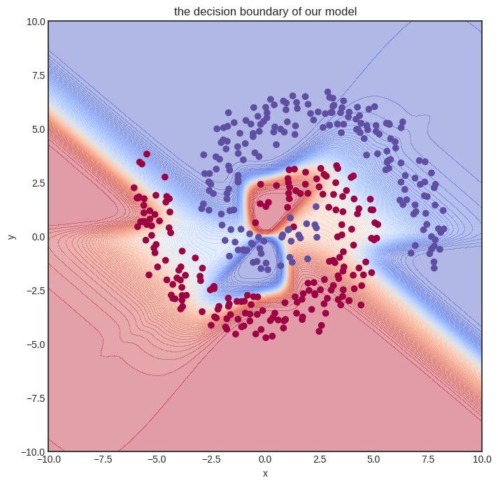
And this is the final result.
visualize_model(model, xs, ys)
/tmp/ipykernel_1198/4170422174.py:15: DeprecationWarning: Conversion of an array with ndim > 0 to a scalar is deprecated, and will error in future. Ensure you extract a single element from your array before performing this operation. (Deprecated NumPy 1.25.)
  zz[i, j] = model.forward(Tensor([xx[i, j], yy[i, j]])).value
Tensor vs Scalar performance comparison#
Before moving on to the implementation details, let’s quickly compare the performance of Scalar vs. Tensor. To do that, we’ll use a simple one-layer neural network with thirty-two hidden neurons.
We’ll store the number of hidden neurons inside a variable so you can play around with it if you execute this notebook locally.
n_hidden_neurons = 32
First, here’s the data. Feel free to skip the code, it’s nothing we haven’t seen before.
import numpy as np
from mlfz.nn.scalar import Scalar
from mlfz.nn.tensor import Tensor

n_samples = 1000

xs_scalar = [[Scalar.from_random(), Scalar.from_random()] for _ in range(n_samples)]
ys_scalar = [Scalar.from_random() for _ in range(n_samples)]

xs_tensor = Tensor(np.array([[x1.value, x2.value] for x1, x2 in xs_scalar]))
ys_tensor = Tensor(np.array([y.value for y in ys_scalar]).reshape(-1, 1))
Our Scalar network takes quite a while to set up. Here we go:
from mlfz import Model
from mlfz.nn.scalar import functional as f_scalar
from itertools import product


class ScalarNetwork(Model):
    def __init__(self):
        self.A = [[Scalar.from_random() for j in range(n_hidden_neurons)]
                  for i in range (2)]
        self.B = [Scalar.from_random() for i in range(n_hidden_neurons)]

    def forward(self, x):
        fs = [sum([self.A[i][j] * x[i] for i in range(2)]) for j in range(n_hidden_neurons)]
        fs_relu = [f_scalar.tanh(f) for f in fs]
        gs = sum([self.B[i] * fs_relu[i] for i in range(n_hidden_neurons)])
        return f_scalar.sigmoid(gs)

    def parameters(self):
        A_dict = {f"a{i}{j}": self.A[i][j] for i, j in product(range(2), range(n_hidden_neurons))}
        B_dict = {f"b{i}": self.B[i] for i in range(n_hidden_neurons)}
        return {**A_dict, **B_dict}
To accurately measure the time of a single gradient step, we encapsulate all the logic into a single function called scalar_network_step.
from mlfz.nn.scalar.loss import binary_cross_entropy as bce_scalar


scalar_net = ScalarNetwork()


def scalar_network_step():
    preds = [scalar_net(x) for x in xs_scalar]
    l = bce_scalar(preds, ys_scalar)
    l.backward()
    scalar_net.gradient_update(0.01)
Let’s go and %timeit!
%timeit scalar_network_step()
---------------------------------------------------------------------------
TypeError                                 Traceback (most recent call last)
Cell In[14], line 1
----> 1 get_ipython().run_line_magic('timeit', 'scalar_network_step()')

File ~/checkouts/readthedocs.org/user_builds/mlfz/envs/latest/lib/python3.10/site-packages/IPython/core/interactiveshell.py:2482, in InteractiveShell.run_line_magic(self, magic_name, line, _stack_depth)
   2480     kwargs['local_ns'] = self.get_local_scope(stack_depth)
   2481 with self.builtin_trap:
-> 2482     result = fn(*args, **kwargs)
   2484 # The code below prevents the output from being displayed
   2485 # when using magics with decorator @output_can_be_silenced
   2486 # when the last Python token in the expression is a ';'.
   2487 if getattr(fn, magic.MAGIC_OUTPUT_CAN_BE_SILENCED, False):

File ~/checkouts/readthedocs.org/user_builds/mlfz/envs/latest/lib/python3.10/site-packages/IPython/core/magics/execution.py:1209, in ExecutionMagics.timeit(self, line, cell, local_ns)
   1207 for index in range(0, 10):
   1208     number = 10 ** index
-> 1209     time_number = timer.timeit(number)
   1210     if time_number >= 0.2:
   1211         break

File ~/checkouts/readthedocs.org/user_builds/mlfz/envs/latest/lib/python3.10/site-packages/IPython/core/magics/execution.py:174, in Timer.timeit(self, number)
    172 gc.disable()
    173 try:
--> 174     timing = self.inner(it, self.timer)
    175 finally:
    176     if gcold:

File <magic-timeit>:1, in inner(_it, _timer)

Cell In[13], line 9, in scalar_network_step()
      7 def scalar_network_step():
      8     preds = [scalar_net(x) for x in xs_scalar]
----> 9     l = bce_scalar(preds, ys_scalar)
     10     l.backward()
     11     scalar_net.gradient_update(0.01)

File ~/checkouts/readthedocs.org/user_builds/mlfz/envs/latest/lib/python3.10/site-packages/mlfz/nn/scalar/loss.py:35, in binary_cross_entropy(preds, ys)
     22 """
     23 Computes the binary cross entropy loss between the predictions and the ground truth.
     24
   (...)
     30     float: The binary cross entropy loss between the predictions and the ground truth.
     31 """
     32 epsilon = 1e-16
     34 return -sum(
---> 35     [
     36         y * log(p + epsilon) + (1 - y) * log(1 - p + epsilon)
     37         for p, y in zip(preds, ys)
     38     ]
     39 ) / len(preds)

File ~/checkouts/readthedocs.org/user_builds/mlfz/envs/latest/lib/python3.10/site-packages/mlfz/nn/scalar/loss.py:36, in <listcomp>(.0)
     22 """
     23 Computes the binary cross entropy loss between the predictions and the ground truth.
     24
   (...)
     30     float: The binary cross entropy loss between the predictions and the ground truth.
     31 """
     32 epsilon = 1e-16
     34 return -sum(
     35     [
---> 36         y * log(p + epsilon) + (1 - y) * log(1 - p + epsilon)
     37         for p, y in zip(preds, ys)
     38     ]
     39 ) / len(preds)

TypeError: unsupported operand type(s) for +: 'NoneType' and 'float'
Now, about the Tensor network.
from mlfz.nn.tensor import functional as f_tensor


class TensorNetwork(Model):
    def __init__(self):
        self.A = Tensor.from_random(2, n_hidden_neurons)
        self.B = Tensor.from_random(n_hidden_neurons, 1)

    def forward(self, x):
        return f_tensor.sigmoid(f_tensor.tanh(x @ self.A) @ self.B)

    def parameters(self):
        return {"A": self.A, "B": self.B}
Look at that simplicity! Vectorization is worth it for that alone, but wait until we see how fast it is.
from mlfz.nn.tensor.loss import binary_cross_entropy as bce_tensor


tensor_net = TensorNetwork()


def tensor_network_step():
    preds = tensor_net(xs_tensor)
    l = bce_tensor(preds, ys_tensor)
    l.backward()
    tensor_net.gradient_update(0.01)
%timeit tensor_network_step()
---------------------------------------------------------------------------
TypeError                                 Traceback (most recent call last)
Cell In[17], line 1
----> 1 get_ipython().run_line_magic('timeit', 'tensor_network_step()')

File ~/checkouts/readthedocs.org/user_builds/mlfz/envs/latest/lib/python3.10/site-packages/IPython/core/interactiveshell.py:2482, in InteractiveShell.run_line_magic(self, magic_name, line, _stack_depth)
   2480     kwargs['local_ns'] = self.get_local_scope(stack_depth)
   2481 with self.builtin_trap:
-> 2482     result = fn(*args, **kwargs)
   2484 # The code below prevents the output from being displayed
   2485 # when using magics with decorator @output_can_be_silenced
   2486 # when the last Python token in the expression is a ';'.
   2487 if getattr(fn, magic.MAGIC_OUTPUT_CAN_BE_SILENCED, False):

File ~/checkouts/readthedocs.org/user_builds/mlfz/envs/latest/lib/python3.10/site-packages/IPython/core/magics/execution.py:1209, in ExecutionMagics.timeit(self, line, cell, local_ns)
   1207 for index in range(0, 10):
   1208     number = 10 ** index
-> 1209     time_number = timer.timeit(number)
   1210     if time_number >= 0.2:
   1211         break

File ~/checkouts/readthedocs.org/user_builds/mlfz/envs/latest/lib/python3.10/site-packages/IPython/core/magics/execution.py:174, in Timer.timeit(self, number)
    172 gc.disable()
    173 try:
--> 174     timing = self.inner(it, self.timer)
    175 finally:
    176     if gcold:

File <magic-timeit>:1, in inner(_it, _timer)

Cell In[16], line 9, in tensor_network_step()
      7 def tensor_network_step():
      8     preds = tensor_net(xs_tensor)
----> 9     l = bce_tensor(preds, ys_tensor)
     10     l.backward()
     11     tensor_net.gradient_update(0.01)

File ~/checkouts/readthedocs.org/user_builds/mlfz/envs/latest/lib/python3.10/site-packages/mlfz/nn/tensor/loss.py:35, in binary_cross_entropy(preds, ys)
     22 """
     23 Computes the binary cross entropy loss between the predictions and the ground truth.
     24
   (...)
     30     float: The binary cross entropy loss between the predictions and the ground truth.
     31 """
     33 epsilon = 1e-16
---> 35 return -(ys * log(preds + epsilon) + (1 - ys) * log(1 - preds + epsilon)).mean()

TypeError: unsupported operand type(s) for +: 'NoneType' and 'float'
The actual performance depends on the server this notebook is built on, but you should see a roughly 100x speedup, given by the magic of vectorization. If you are running this notebook locally, try changing the n_hidden_neurons variable in the first executable cell in this notebook. You’ll be surprised: the execution time of the Scalar version will rapidly increase, but the Tensor version will roughly stay the same!
That’s because the graph structure adds a heavy overhead to our computations. We’ll profile the code in a later version of the notebook, but this is because the actual computations like addition, multiplication, etc, are only a small portion of the training!