Building a neural network

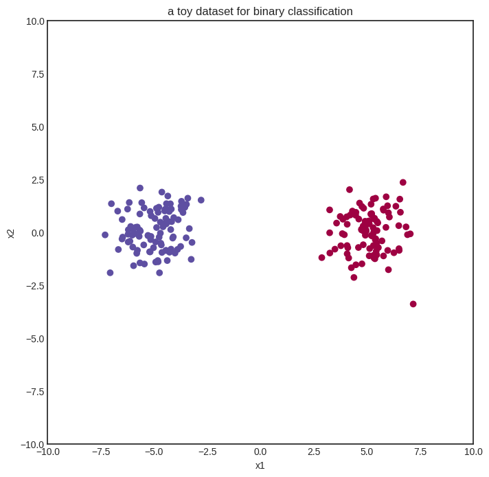
We start with a simple binary classification problem to demonstrate how neural networks work. Here’s our (generated) dataset of two blue and red classes encoded with 0 and 1.

import random
import matplotlib.pyplot as plt


xs = [(random.normalvariate(0, 1) - 5 , random.normalvariate(0, 1)) for _ in range(100)] \
    + [(random.normalvariate(0, 1) + 5 , random.normalvariate(0, 1)) for _ in range(100)]
ys = [1 for _ in range(100)] + [0 for _ in range(100)]

Show code cell source Hide code cell source

with plt.style.context("seaborn-v0_8-white"):
    plt.figure(figsize=(8, 8))
    plt.xlim([-10, 10])
    plt.ylim([-10, 10])
    plt.scatter([x[0] for x in xs], [x[1] for x in xs], c=ys, cmap=plt.cm.Spectral)
    plt.title("a toy dataset for binary classification")
    plt.xlabel("x1")
    plt.ylabel("x2")
    plt.show()

We’ll start with the simplest neural network: zero hidden layers and sigmoid activation. This is also known as logistic regression. Here we go:

from mlfz.nn import Model
from mlfz.nn.scalar import Scalar, sigmoid, binary_cross_entropy


class ZeroLayerNetwork(Model):
    def __init__(self):
        self.a1 = Scalar(1)
        self.a2 = Scalar(1)
        self.b = Scalar(1)

    def forward(self, x):
        x1, x2 = x
        return sigmoid(self.a1 * x1 + self.a2 * x2 + self.b)
    
    def parameters(self):
        return {"a1": self.a1, "a2": self.a2, "b": self.b}

model = ZeroLayerNetwork()

We can visualize the untrained model on a heatmap, coloring according to predictions.

Show code cell source Hide code cell source

import numpy as np


def visualize_model(model, xs, ys, res=100, xrange=(-10, 10), yrange=(-10, 10)):
    with plt.style.context("seaborn-v0_8-white"):
        plt.figure(figsize=(8, 8))
        
        res = 100
        x = np.linspace(xrange[0], xrange[1], res)
        y = np.linspace(yrange[0], yrange[1], res)
        xx, yy = np.meshgrid(x, y)
        
        zz = np.vectorize(lambda x, y: model((x, y)).value)(xx, yy)

        # plot the decision boundary
        plt.contourf(xx, yy, zz, levels=100, cmap='coolwarm_r', alpha=0.4)
        plt.xlabel('x')
        plt.ylabel('y')
        plt.title('the decision boundary of our model')
        
        # plot the data
        plt.scatter([x[0] for x in xs], [x[1] for x in xs], c=ys, cmap=plt.cm.Spectral, zorder=10)
        plt.show()


visualize_model(model, xs, ys)

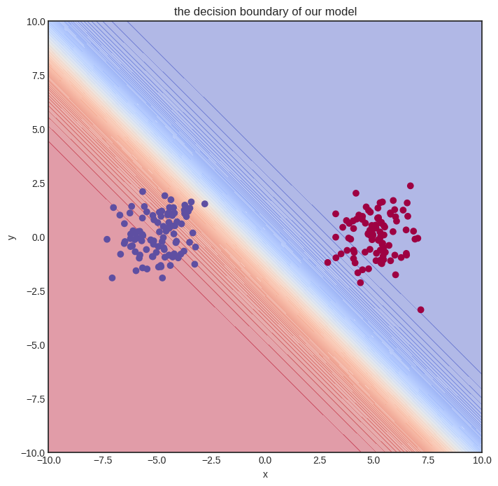
The initial model gets nothing right, so let’s train it!

n_steps = 100
lr = 0.1

for i in range(1, n_steps + 1):
    preds = [model(x) for x in xs]
    l = binary_cross_entropy(preds, ys)
    l.backward()
    model.gradient_update(lr)

    if i == 1 or i % 10 == 0:
        print(f"step no. {i}, loss = {l.value}")

step no. 1, loss = 5.025041985167245
step no. 10, loss = 0.07125507955417765

step no. 20, loss = 0.029065634451322642
step no. 30, loss = 0.01840495328853839

step no. 40, loss = 0.013529241137846967
step no. 50, loss = 0.010726888845382278

step no. 60, loss = 0.008903711674840472

step no. 70, loss = 0.007621011921518769
step no. 80, loss = 0.006668455849913537

step no. 90, loss = 0.005932497820554603
step no. 100, loss = 0.005346406531361452

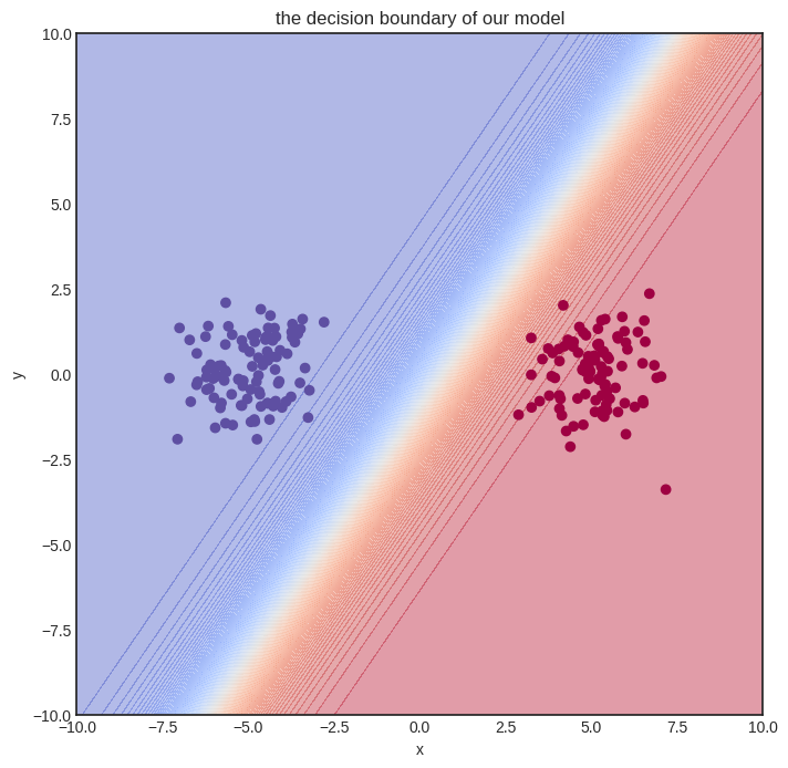
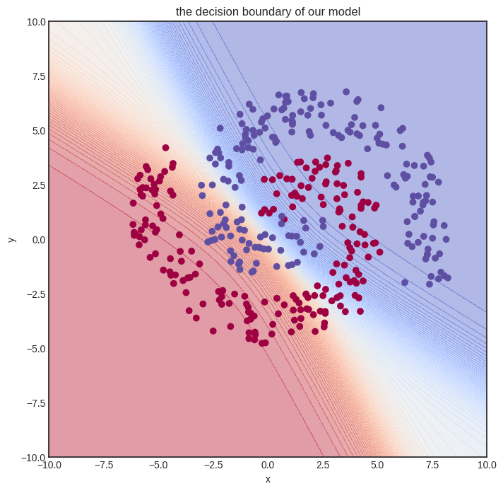
Here’s how the model performs after training.

Show code cell source Hide code cell source

visualize_model(model, xs, ys)

Solving a simple problem like that is no big deal. Can we handle more complex datasets?

A multi-layer network

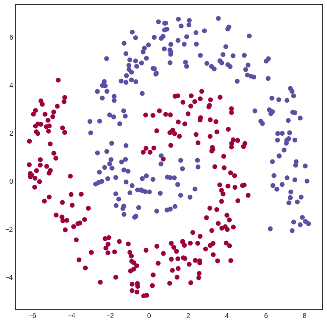
Here’s a spiral-like dataset with classes intertwined into each other.

Show code cell source Hide code cell source

import math


def generate_spiral_dataset(n_points, noise=0.5, twist=380):
    random_points = [math.sqrt(random.random()) * twist * 2 * math.pi/360 for _ in range(n_points)]

    class_1 = [(-math.cos(p) * p + random.random()*noise, math.sin(p) * p + random.random()*noise) for p in random_points]
    class_2 = [(math.cos(p) * p + random.random()*noise, -math.sin(p) * p + random.random()*noise) for p in random_points]

    xs = class_1 + class_2
    ys = [0 for _ in class_1] + [1 for _ in class_2]
    
    return xs, ys

xs, ys = generate_spiral_dataset(200, noise=2)

Show code cell source Hide code cell source

with plt.style.context("seaborn-v0_8-white"):
    plt.figure(figsize=(8, 8))
    plt.scatter([x[0] for x in xs], [x[1] for x in xs], c=ys, cmap=plt.cm.Spectral)
    plt.show()

For this problem, we need a hidden layer. Here’s a model with a hidden layer of eight neurons, connected via the

\[ \mathrm{tanh}(x) = \frac{e^{2x} - 1}{e^{2x} + 1} \]

activation function.

from mlfz.nn.scalar import tanh
from itertools import product


class OneLayerNetwork(Model):
    def __init__(self):
        self.A = [[Scalar.from_random() for j in range(4)]
                  for i in range (2)]
        self.B = [Scalar.from_random() for i in range(4)]
    
    def forward(self, x):
        """
        x: a tuple of two Scalars
        """
        fs = [sum([self.A[i][j] * x[i] for i in range(2)]) for j in range(4)]
        fs_relu = [tanh(f) for f in fs]
        gs = sum([self.B[i] * fs_relu[i] for i in range(4)])
        return sigmoid(gs)

    def parameters(self):
        A_dict = {f"a{i}{j}": self.A[i][j] for i, j in product(range(2), range(4))}
        B_dict = {f"b{i}": self.B[i] for i in range(4)}
        return {**A_dict, **B_dict}

We can already see one of the glaring flaws of our Scalar implementation of computational graphs: the inability to write vectorized code. For instance, the expression

fs = [sum([self.A[i][j] * x[i] for i in range(2)]) for j in range(4)]

is simply the matrix product of the input x and the \( 2 \times 4 \) parameter matrix A.

We’ll deal with vectorization later with the Tensor class, but let’s stick to the vanilla version for now. Here’s our model.

model = OneLayerNetwork()

And here’s how the untrained model looks.

Show code cell source Hide code cell source

visualize_model(model, xs, ys)

Let’s train it! We’ll need quite some more steps. To spice things up, we’ll also use a simple learning rate tuning: lr=1 for the first hundred gradient descent steps, lr=0.5 for the second hundred, and lr=0.1 after.

n_steps = 1000
lr = 0.2

for i in range(1, n_steps + 1):
    preds = [model(x) for x in xs]
    l = binary_cross_entropy(preds, ys)
    l.backward()
    model.gradient_update(lr)

    if i == 1 or i % 100 == 0:
        print(f"step no. {i}, loss = {l.value}")

step no. 1, loss = 0.6421108496937449

step no. 100, loss = 0.5415495017511247

step no. 200, loss = 0.49626749234829115

step no. 300, loss = 0.47698455858939426

step no. 400, loss = 0.46502265852896363

step no. 500, loss = 0.4563883276075638

step no. 600, loss = 0.4485039041770576

step no. 700, loss = 0.4717202520255668

step no. 800, loss = 0.4536386186247771

step no. 900, loss = 0.4516829500601066

step no. 1000, loss = 0.4502377052139057

This training took a while to execute on my Lenovo Thinkpad and probably much more on the Read the Docs servers. (My apologies.) Again, this is the consequence of non-vectorized code. Is the model any good? Let’s see.

Show code cell source Hide code cell source

visualize_model(model, xs, ys)

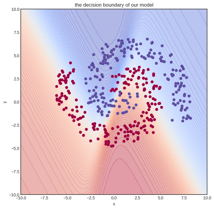
Eh. Not perfect at all, but we can already see that the decision boundary is starting to conform to the data. We need a more expressive model and more training iterations. Sadly, this is not possible due to build time restrictions. Remember that this interactive book is pre-built on Read the Docs servers, with fifteen minutes of total build time.

This hiccup foreshadows the need for more effective code, which we’ll bring to fruition with vectorization.

But let’s not get ahead of ourselves and see how Scalar works on the inside! Trust me on this: understanding plain scalar-valued computational graphs is paramount to building hyper-fast vectorized ones. We dial up the difficulty one notch at a time, and right now, the next step is digging deep into the forward pass.