Model: training neural networks#
To train a neural network in mlfz, you should use the Model class, which provides a convenient interface to interact with computational graphs.
It’s best to provide an example, so here we go!
from mlfz.nn.scalar import Scalar
from mlfz.nn import Model


class Linear(Model):
    def __init__(self):
        self.a = Scalar(1)
        self.b = Scalar(1)

    def forward(self, x):
        return self.a * x + self.b

    def parameters(self):
        return {"a": self.a, "b": self.b}
Each Model subclass has two key methods that you have to implement: forward and parameters. forward defines the computational graph and acts as a callable that turns inputs into predictions, while parameters enumerate the Scalars that have to be updated during gradient descent.
Let’s see our model in action!
linear = Linear()

linear.forward(2)
Scalar(3)
Model instances are callable, and the function call operator is just a shortcut to the forward method.
linear(2)
Scalar(3)
linear.parameters()
{'a': Scalar(1), 'b': Scalar(1)}
This is a good time to highlight that scalar operations work with vanilla number types, like integers, floats, whatever. It’s just for convenience, saving us from typing Scalar(...) all the time.
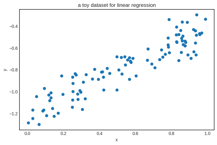
To train this simple model, we’ll generate a toy dataset from the target function \( h(x) = 0.8 x - 1.2 \).
from random import random, normalvariate


xs = [random() for _ in range(100)]
ys = [0.8*x - 1.2 + normalvariate(0, 0.1) for x in xs]
Show code cell source
import matplotlib.pyplot as plt


with plt.style.context("seaborn-v0_8-white"):
    plt.figure(figsize=(8, 5))
    plt.scatter(xs, ys)
    plt.xlabel('x')
    plt.ylabel('y')
    plt.title('a toy dataset for linear regression')
    plt.show()
We’ll also need a loss function as well. Let’s go with the simplest one: the mean squared error, defined by the formula
where \( \widehat{\mathbf{y}} \in \mathbb{R}^N \) is the vector of predictions, while \( \mathbf{y} \in \mathbb{R}^N \) is the vector of ground truths.
from mlfz.nn.scalar.loss import mean_squared_error


preds = [linear(x) for x in xs]
mean_squared_error(preds, ys)
Scalar(5.411656067863613)
We have everything ready to train our model with gradient descent.
n_steps = 100
lr = 0.2


for i in range(1, n_steps + 1):
    preds = [linear(x) for x in xs]
    l = mean_squared_error(preds, ys)
    l.backward()
    linear.gradient_update(lr=lr)

    if i == 1 or i % 10 == 0:
        print(f"step no. {i}, loss = {l.value}")
step no. 1, loss = 5.411656067863613
step no. 10, loss = 0.04426991198506776
step no. 20, loss = 0.02939643646102766
step no. 30, loss = 0.02087579178681936
step no. 40, loss = 0.015992183347117394
step no. 50, loss = 0.013193142627762937
step no. 60, loss = 0.01158887212873774
step no. 70, loss = 0.010669384314128134
step no. 80, loss = 0.01014237977111043
step no. 90, loss = 0.009840327058775987
step no. 100, loss = 0.00966720551317002
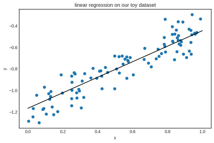
Here’s the result.
linear.parameters()
{'a': Scalar(0.7222919030024763), 'b': Scalar(-1.1694743421955895)}
Looks good! The parameters seem close to the target function \( h(x) = 0.8x - 1.2 \). Here’s the plot.
Show code cell source
with plt.style.context("seaborn-v0_8-white"):
    plt.figure(figsize=(8, 5))

    xs_plot = [0.01 * k for k in range(101)]
    ys_plot = [linear(x).value for x in xs_plot]
    plt.plot(xs_plot, ys_plot, c="k")

    plt.scatter(xs, ys)
    plt.xlabel('x')
    plt.ylabel('y')
    plt.title('linear regression on our toy dataset')
    plt.show()
Optimizers#
Although training a model using vanilla gradient descent doesn’t require more than five lines of code, ready-made optimizers are available. (For now, only gradient descent is implemented, but more will come, including stochastic gradient descent, Adagrad, and others.)
from mlfz.nn.scalar.optimizer import GradientDescent


linear = Linear()
optimizer = GradientDescent(model=linear, loss_fn=mean_squared_error)
optimizer.run(xs, ys, lr=0.1, n_steps=1000)
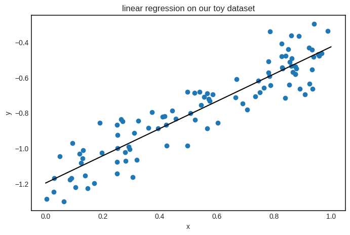
The result is the same. Check it out:
linear.parameters()
{'a': Scalar(0.7711109331787215), 'b': Scalar(-1.1981267209202828)}
Show code cell source
with plt.style.context("seaborn-v0_8-white"):
    plt.figure(figsize=(8, 5))

    xs_plot = [0.01 * k for k in range(101)]
    ys_plot = [linear(x).value for x in xs_plot]
    plt.plot(xs_plot, ys_plot, c="k")

    plt.scatter(xs, ys)
    plt.xlabel('x')
    plt.ylabel('y')
    plt.title('linear regression on our toy dataset')
    plt.show()
Saving and loading parameters#
Let’s go back to square one. The Model class allows you to save and load parameters dynamically.
linear = Linear()

linear.parameters()
{'a': Scalar(1), 'b': Scalar(1)}
linear.load_parameters({"a": Scalar(-1), "b": Scalar(-1)})
linear.parameters()
{'a': Scalar(-1), 'b': Scalar(-1)}
If you need the parameters in a vanilla Python version, just use the Model.parameter_values method.
linear.parameter_values()
{'a': -1, 'b': -1}
Keep in mind that in Python, Scalar objects are stored by reference, unlike, say, a Python float. This means that if you save the parameter dictionary and then use gradient descent to tune the parameters, your saved parameter dictionary will also change. Take a look.
print("using Model.parameters():")
linear = Linear()
p = linear.parameters()
print(f"before: p = {p}")

preds = [linear(x) for x in xs]
l = mean_squared_error(preds, ys)
l.backward()
linear.gradient_update(lr=10)
print(f"after: p = {p}")
using Model.parameters():
before: p = {'a': Scalar(1), 'b': Scalar(1)}
after: p = {'a': Scalar(-24.8143897811932), 'b': Scalar(-45.46492520169118)}
To avoid issues from this, we can use the Model.copy_parameters method.
print("using Model.copy_parameters():")
linear = Linear()
p = linear.copy_parameters()
print(f"before: p = {p}")

preds = [linear(x) for x in xs]
l = mean_squared_error(preds, ys)
l.backward()
linear.gradient_update(lr=10)
print(f"after: p = {p}")
using Model.copy_parameters():
before: p = {'a': Scalar(1), 'b': Scalar(1)}
after: p = {'a': Scalar(1), 'b': Scalar(1)}
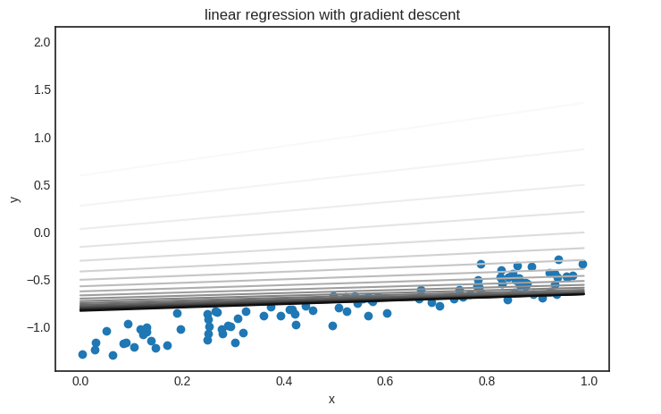
Parameter saving and loading are useful if you want to visualize the model’s state during training. Here’s an example demonstrating how gradient descent fits a linear regression model.
linear = Linear()

n_steps = 200
lr = 0.01

parameter_list = [linear.copy_parameters()]

for _ in range(n_steps):
    preds = [linear(x) for x in xs]
    l = mean_squared_error(preds, ys)
    l.backward()
    linear.gradient_update(lr)
    parameter_list.append(linear.copy_parameters())
Show code cell source
from matplotlib import colormaps

color_map = colormaps['Greys']

with plt.style.context('seaborn-v0_8-white'):
    plt.figure(figsize=(8, 5))
    plt.scatter(xs, ys)

    xs_plot = [k*0.01 for k in range(100)]

    trimmed_parameter_list = parameter_list[::10]
    for i, params in enumerate(trimmed_parameter_list):
        color = color_map(i / len(trimmed_parameter_list))
        linear.load_parameters(params)
        ys_plot = [linear(x).value for x in xs_plot]
        plt.plot(xs_plot, ys_plot, color=color)

    plt.title("linear regression with gradient descent")
    plt.xlabel("x")
    plt.ylabel("y")
    plt.legend(bbox_to_anchor=(1.05, 0.0), loc='lower left')
    plt.show()
/tmp/ipykernel_940/2321412048.py:21: UserWarning: No artists with labels found to put in legend.  Note that artists whose label start with an underscore are ignored when legend() is called with no argument.
  plt.legend(bbox_to_anchor=(1.05, 0.0), loc='lower left')
It’s time to see an actual neural network!